Written by Andy
One thing that many high school students struggle with in the study of probability is the topic of conditional probability, and, in particular, the difference between mutually exclusive and independent events. To define these, let us begin by reviewing some of the basic definitions in the study of probability. Consider an experiment, such as rolling a 6-sided die, in which the outcome of a particular trial cannot be predicted with certainty, but for which the set of all possible outcomes is known and can be listed. This set is known as the sample space associated to the experiment. For the example of rolling a die, each possible outcome is a positive integer from 1 to 6, so the sample space is the set S = {1,2,3,4,5,6}. An event is a subset of the sample space. For example, the events of rolling a 2, rolling an even number, and rolling a prime number are, respectively, {2}, {2,4,6}, and {2,3,5}. The study of probability is concerned with quantifying the “chance” that an event A occurs. One way to do this is to simply repeat the experiment a large number of times, and count the number of times that the event A occurs (i.e., the number of times the outcome belongs to the event A). If n is the number of times the experiment is repeated and N(A) the number of times which A occurs, then the relative frequency R(A) ≡ N(A)/n is the fraction of the time that A occurs in the n trials. Since n > 0 and 0 ≤ N(A) ≤ n , the relative frequency lies in the range 0 ≤ R(A) ≤ 1. In the graph below, we plot the relative frequency of rolling a 6 on a standard 6-sided die. Don’t worry about the units in the Y axis, which represent the relative frequency of the selected outcome – that is, the number of times you rolled a 2 (say) out of the total number of rolls. Basically we need only pay attention to what the graph shows qualitatively, which is that the line flattens out as n increases.
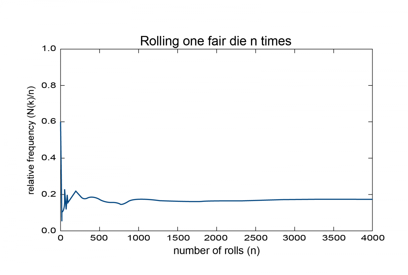
As we see, the relative frequency is very unstable for small values of n (if you roll a die twice and get a 1 on the first roll and then then a 6 on the second, the relative frequency for these two trials jumps from 0 to 1/2!), but stabilizes as n becomes large (this is known as the “law of large numbers”). Thus, the relative frequency R(A) is an approximation to the true probability of A, which becomes better and better as n becomes larger. We therefore define the probability of the event A as the number the relative frequency of A approaches and would reach if we could do an infinite number of trials. We denote this by

More formally, we can view P(A) as a function which assigns to each event A a real number. To be interpreted as a probability, this function must satisfy three properties. The first two are very intuitive, if you think about the definition above:
1. P(A) ≥ 0 for every event A. (Probabilities cannot be negative.)
2. P(S) = 1 (The outcome is certain to lie in the sample space.)
To state the third, first recall that the union of two sets A and B is the set
A ⋃ B = {x : x belongs to at least one of the sets A or B} and the intersection of A and B is the set
A ⋂ B = {x : x belongs to both the sets A and B} . If A and B have no elements in common, then their intersection is the empty set (which is defined to be the unique set with no elements), and we write A ⋂ B = φ . For example, if A = {1,3,5}, B={2,4,6}, and C={1,2,3}, then A ⋃ B = {1, 2, 3, 4, 5, 6} , A ⋂ C = {1, 3} , and A ⋂ B = φ . The third property of the function P can now be stated:
3. If A and B are any two events events such that A ⋂ B = φ , then
P(A ⋃ B) = P(A) + P(B) .
Two events such that A ⋂ B = φ are said to be mutually exclusive, as it is impossible that they both occur at the same time (i.e., there is no way that the outcome of an experiment can be in both A and B at the same time, since there is nothing in their intersection). Going back to the die example, the events A={1,3,5} and B={2,4,6} are mutually exclusive, since the outcome of a roll can’t be both even and odd. In words, Property 3 says that the probability of the union of two mutually exclusive events is the sum of their individual probabilities. To see that this property is implied by our definition of probability above, note that if A ⋂ B = φ , then the number of elements in A ⋃ B is the sum of the number of elements in A and the number of elements in B. The definition of P above then gives
![]()
This property can be extended to unions of more than two events: if all the events are mutually exclusive, then the probability of the union is the sum of the probabilities of all these events.
Any function P satisfying these three properties is called a probability set function. From these properties, one can prove various other important properties of P. The most useful of these are
•P(φ) = 0.
•For any event A, 0 ≤ P(A) ≤ 1 .
- •For any events A and B, P(A ⋃ B) = P(A) + P(B) − P(A ⋂ B) .
Note that the last of these reduces to property 3 above when A ⋂ B = φ , since P(φ) = 0 .
Let us now return to our example of a fair die. Since the events {1},…,{6} are mutually exclusive (you can only get one of these outcomes on a given roll) and all are equally likely (since the die is fair), properties 1 and 3 give P(S) = P({1} ⋃ {2} ⋃ … ⋃ {6}) = P({1}) + P({2}) + … + P({6}) =6 P({i}) = 1 , we have P({i}) = 1/6 for all i = 1, …, 6 , as one would expect. Note that this method of assigning the probability did not depend on any observations. Instead, we deduced this from the assumption that all outcomes were equally likely. Probabilities assigned this way are called theoretical probabilities. If one’s assumptions are accurate, then the empirical probability should agree with the theoretical probability. More generally, under the assumption that every outcome in the sample space is equally likely, a similar derivation shows that

where |A| denotes the number of elements in the set A.
Let us now discuss conditional probability. Suppose now you are playing a game in which you flip two fair coins. The sample space is S={HH,HT,TH,TT}. Consider the following events: A={HH,HT} (heads on the first coin), B={HT,TT} (tails on the second coin), C={TT} (tails on both coins). This game works as follows: you begin by placing a bet on a particular event. Then, after flipping the coins, you receive an additional piece of information, after which you are allowed to place an additional bet, if you wish. Suppose you place your initial bet on the event B. After flipping the coins you are told that event C occurred, and asked if you would like to increase your bet. Since you are now certain that B occurred (if both coins landed tails, in particular the second coin landed tails), you confidently increase your bet. Note that the additional information increased the probability that B occurred from 2/4=1/2 to 1. Suppose you flip again and this time you are told that A occurred, and again asked if you would like to increase your original bet. Since the outcome of the first coin has no effect on the outcome of the second, in this case the additional information that A occurred does not increase the probability of B, so there is no reason to increase the initial bet.
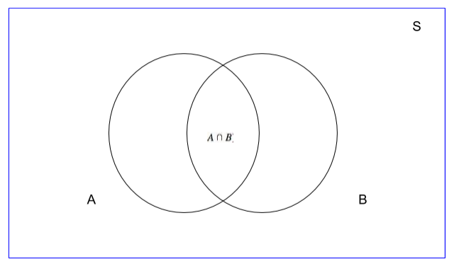
The game just described illustrates a common situation: before you know the outcome of an experiment, sometimes you obtain additional information, which changes the probability of the original event. The new probability of an event A, given that another event B occurred, is called the conditional probability of A given B, and denoted P(A|B) . To compute the conditional probability of A given B, you treat B as the “new” sample space, since you now know that the outcome of the experiment must belong to B. Then, if A still occurred, the outcome must belong to the overlap of A and B, i.e., their intersection. Thus, the formula for the conditional probability is

This can be visualized by the Venn diagram below. Geometrically, one can P(B) P(A⋂B) view P(A) as the fraction of the area of the sample space S taken up by A. If we take B to be the new sample space, then the new probability of A (the conditional probability), is the fraction of the area of B taken up by A, which is precisely A ⋂ B .
It is straightforward to check that the function assigning to A its conditional probability P(A|B) is a valid probability set function, i.e., that it satisfies properties 1-3 above. Thus, all the properties which follow from these, including the ones listed above, continue to hold for conditional probabilities, just as for ordinary probabilities.
Let us verify that the formula just given indeed reproduces the correct conditional probabilities for the events in the coin flipping game described above. First, note that A ⋂ B = {HT} and B ⋂ C = {TT} . From these, we calculate
![]() ,
,
while
![]() .
.
As we noticed above, the outcome of the first coin in no way affects the outcome of the second coin, so the probability of A is unchanged. In general, two events A and B are said to be independent if
![]() .
.
This equation quantifies what it means for two events to have no influence on each other. Another useful way of characterizing independent events A and B is given by first rearranging the defining equation for conditional probability as P(A ⋂ B) = P(A|B)P(B) and then using the fact that if A and B are independent, then P(A|B) = P(A) . Substituting then gives P(A ⋂ B) = P(A)P(B) , which says that two events A and B are independent if and only if their joint probability is equal to the product of their individual probabilities.
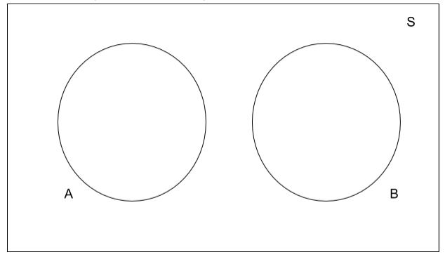
Let us now discuss the difference between mutual exclusivity and independence. Let A and B be two non-empty events (if one of the events is empty, then it has zero probability of occurring, so this is not very interesting). If A and B are mutually exclusive, then P(A ⋂ B) = P(φ) = 0. However, since A and B are both non-empty, P(A) and P(B) are both greater than zero, so their product P(A)P(B)>0, since the product of positive numbers is always positive. Thus, we see that if A and B are mutually exclusive, then P(A ⋂ B) =/ P(A)P(B) hence they are not independent! This can again be easily visualized by using Venn diagrams. The Venn diagram below shows two mutually exclusive non-empty events A and B. Since their intersection is empty, the two circles are disjoint.
Since A is non-empty, P(A)>0. If you are now told that B has occurred, then the conditional
probability of A given by is

Thus, now that we know B has occurred, we know for certain that A did not occur, hence the probability of A drops to 0. This shows that any pair of non-empty mutually exclusive events is never independent.
Be sure to give us a shout if you have any questions!